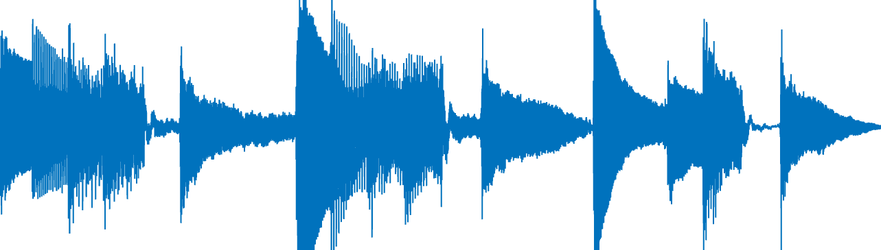
Alright, so you’re out one evening and you see a fantastic musician. The live performance sounds clean – like this:
You wish that you could hear those sweet, sweet tunes again. However, you are only armed with a mediocre cell phone recording…
… and the author’s “studio” version, where they added a bunch of effects muddying the original tones.
Is it possible to recover or approximate the original audio tune?
Yes, using the nonlinear recovery framework I developed with Patrick L. Combettes:
How do we do this? Let’s start with a brief detour into audio processing.
Modeling the distortion of sound
The WAV file format typically samples a sound $44,100$ times per second, yielding amplitudes in $[-1,1]$. Since we’re working with a sample which is just over $7$ seconds, we’re living in $\mathbb{R}^{N}$ where $N>308,700$.
Bad recordings
The phenomenon of “clipping” is often modeled via a truncation of amplitude. This is what happens when we clip all of the amplitudes of the original sound $\overline{x}$ to $[-0.05,0.05]$:
Mathematically, we can model this observation process via the projection onto the hypercube $[-0.05,0.05]^N$, i.e., $T_1=\textrm{proj}_{[-0.05,0.05]^N}$. Note that $F_1$ is nonlinear and nonsmooth.
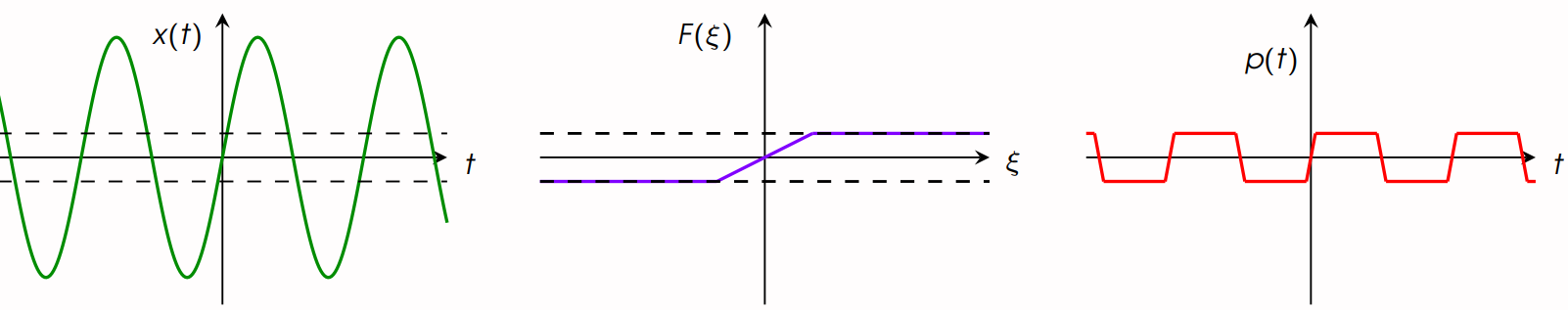
Figure 1: An example of hard clipping. Left to right: Original signal; Characteristic curve of hard-clipping; clipped version of the original signal.
Modeling echo, reverb, and frequency modulation
Next we are going to mathematically model the operation which takes the original sound and outputs this “artistic” sample:
We can hear a few things from this sample:
- Distortion has been added.
- Echo has been added
- It sounds like it has gone through an analogue telephone. Instead of having a full frequency bandwidth, only a subset of frequencies are transmitted, i.e., the signal was bandlimited.
Note: for further details on these models, check out Hack Audio by Eric Tarr.
We can estimate the time duration of the echo (roughly $0.3$ seconds), and model this process using discrete convolution, which I’ll represent with a linear operator $L_{1}$ . Likewise, using a little bit of Fourier analysis, we can encode the process of bandlimit to the frequency range of an analogue telephone ($400$ – $3400$ Hz) via a linear operator $L_{2}$.
Finally, there are two types of nonlinear distortion in this clip – half-wave rectification $F_1$ and soft-clipping arctangent distortion $F_2$. Altogether, we have a superposition of waveforms with all of these effects, shown in the circuit diagram in Figure 2.
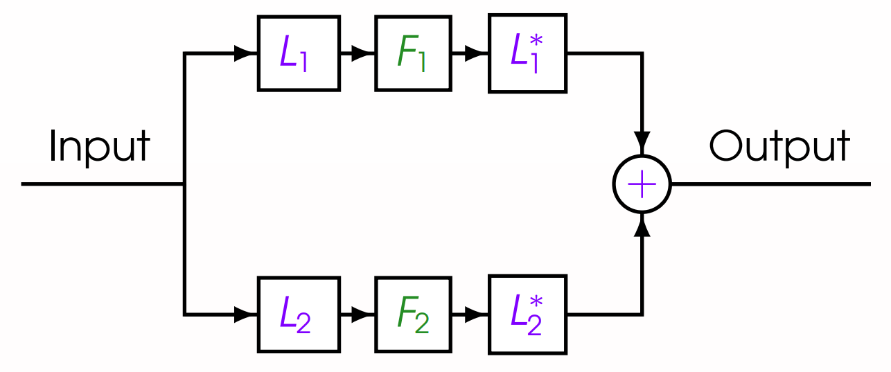
Figure 2: Circuit diagram showing the distortion model.
Concretely, this process is modeled by $T_2 = L_1^\top\circ F_1 \circ L_1 + L_2^\top \circ F_2 \circ L_2$.
Defining the inverse problem
Now that we have our operators, we seek to
\[\text{find}\;\;x\in [-1,1]^N\;\;\text{such that}\;\;T_1x=p_1\;\;\text{and}\;\;T_2x=p_2, \tag{$*$}\]where $p_1=T_1\overline{x}$ and $p_2=T_2\overline{x}$ respectively denote our clipped and distorted observations.
Here's where the math comes in
At first, one may be tempted to solve the following
\[\textrm{minimize}_{x\in[-1,1]^N} \|T_1x-p_1\|^2+\|T_2x-p_2\|^2.\]However, since $T_1$ and $T_2$ are nonlinear operators, we run into some numerical and theoretical issues since the objective function is nonconvex. In general, this miminimization problem is solved iteratively with algorithms which only yield local convergence to a local minimizer.
Nonetheless, there are algorithms which can solve $(*)$ and are proven to converge to a solution from any initial iterate. These algorithms are tractable since they rely on evaluating the forward-operators $T_1$ and $T_2$. It turns out that both $T_1$ and $T_2$ can be described by firmly nonexpansive operators, which exactly fits the nonlinear model described here. (see also here for an extrapolated feasibility algorithm and or here for an extension incase the operators are poorly modeled).
Anyhow, using the modeling and results from this series of papers gives you the following recovery. Thanks for reading, and rock on!
A few implementation notes and random comments:
- If there are no solutions to the inverse problem $(*)$ (e.g., we got the frequency range incorrect, or we incorrectly estimated the echo delay), I would recommend using the algorithm from this paper. It is proven to converge under very mild conditions, even if $(*)$ has no solutions. The point we converge to solves a relaxation of $(*)$. For this specific audio problem, since the hypercube $[-1,1]^N$ is bounded, the algorithm in the paper above is guaranteed to converge.
- To handle the hard constraint $x\in[-1,1]^N$, we have a few options -- one could just rely on the projector which is easily computed. However, if for your problem it's expensive (or impossible) to compute the projection, you can also use a subgradient projector, which is sortof like a subgradient descent-step. These are quite useful if you have hard constraints described by convex lower semicontinuous inequalities, as was done in this article.
- The convergence proof for these algorithms relies heavily on the fact that these nonlinearities are firmly nonexpansive. This is a rather broad class of nonlinear operators which we can use to mathematically model a variety of nonlinearities cropping up in the wild. In fact, even if your operator fails to be firmly nonexpansive, you may be able to solve your problem using the notion of proxification. In short, sometimes by "gluing" discontinuities, rescaling, and applying the occasional adjoint, one can artificially create a firmly nonexpansive operator which equivalently encodes your nonlinear equation.